
Symbolic Regression (sklearn mode)#
Preview#
In this example we will solve the Symbolic Regression problem using Sklearn and EC-KitY.
Setting the experiment#
First, we need to import the components we want to use in our experiment.
Import external modules:
import numpy as np
from time import time

from sklearn.datasets import make_regression
from sklearn.model_selection import train_test_split
from sklearn.metrics import mean_absolute_error
Import internal modules:
from eckity.algorithms.simple_evolution import SimpleEvolution
from eckity.breeders.simple_breeder import SimpleBreeder
from eckity.creators.gp_creators.ramped_hh import RampedHalfAndHalfCreator
from eckity.genetic_encodings.gp.tree.functions import f_add, f_mul, f_sub
from eckity.genetic_encodings.gp.tree.utils import create_terminal_set
from eckity.genetic_operators.crossovers.subtree_crossover import SubtreeCrossover
from eckity.genetic_operators.mutations.erc_mutation import ErcMutation
from eckity.genetic_operators.mutations.subtree_mutation import SubtreeMutation
from eckity.genetic_operators.selections.tournament_selection import TournamentSelection
from eckity.sklearn_compatible.sk_regressor import SKRegressor
from eckity.statistics.best_average_worst_statistics import BestAverageWorstStatistics
from eckity.subpopulation import Subpopulation
from eckity.termination_checkers.threshold_from_target_termination_checker import ThresholdFromTargetTerminationChecker
from eckity.sklearn_compatible.regression_evaluator import RegressionEvaluator
Adding custom functions#
Before creating the experiment we may define custom functions as internal GP Tree nodes. More on this in the function-set section below.
# Adding your own functions
def f_add3(x1, x2, x3):
    return np.add(np.add(x1, x2), x3)


def f_mul3(x1, x2, x3):
    return np.multiply(np.multiply(x1, x2), x3)
Generating a regression problem#
Using scikit-learn, our dataset will be a random regression problem.
# generate a random regression problem
X, y = make_regression(n_samples=500, n_features=5)
Creating the set of tree nodes#
Each node in the GP tree is either a function (internal node) or a terminal (leaf).
Function set#
# function nodes, each has two children (which are its operands)
function_set = [f_add, f_mul, f_sub, f_div, f_sqrt, f_log, f_abs, f_max, f_min, f_inv, f_neg]
Our tree individuals will contain some common mathematical functions as internal nodes.
Terminal set#
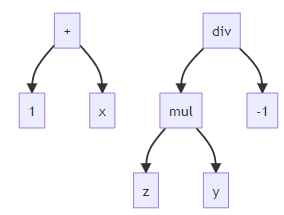
The inner nodes (terminal set) will be the vars x, y, z, or the constant numbers 0, 1 or -1. When EC-KitY is used in sklearn mode, we will generate the terminal set automatically, by referring to the number of features.
# Automatically generate a terminal set.
# Since there are 5 features, set terminal_set to: ['x0', 'x1', 'x2', 'x3', 'x4']
terminal_set = create_terminal_set(X)
An example of two possible individuals:
Initializing the evolutionary algorithm#
The Evolution object is the main part of the experiment. It receives the parameters of the experiment and runs the evolutionary process.
# Initialize Simple Evolutionary Algorithm instance
    algo = SimpleEvolution(
        Subpopulation(creators=RampedHalfAndHalfCreator(init_depth=(2, 4),
                                                        terminal_set=terminal_set,
                                                        function_set=function_set,
                                                        erc_range=(-100, 100),
                                                        bloat_weight=0.0001),
                      population_size=1000,
                      # user-defined fitness evaluation method
                      evaluator=RegressionEvaluator(),
                      # minimization problem (fitness is MAE), so higher fitness is worse
                      higher_is_better=False,
                      elitism_rate=0.05,
                      # genetic operators sequence to be applied in each generation
                      operators_sequence=[
                          SubtreeCrossover(probability=0.9, arity=2),
                          SubtreeMutation(probability=0.2, arity=1),
                          ErcMutation(probability=0.05, arity=1)
                      ],
                      selection_methods=[
                          # (selection method, selection probability) tuple
                          (TournamentSelection(tournament_size=4, higher_is_better=False), 1)
                      ]
                      ),
        breeder=SimpleBreeder(),
        max_workers=1,
        max_generation=1000,
        # optimal fitness is 0, evolution ("training") process will be finished when best fitness <= threshold
        termination_checker=ThresholdFromTargetTerminationChecker(optimal=0, threshold=0.01),
        statistics=BestAverageWorstStatistics()
    )
Let’s break down the parts and understand their meaning.
Initializing Subpopulation#
Sub-population is the object that holds the individuals, and the objects that are responsible for treating them (a Population can include a list of multiple Subpopulations but it is not needed in this case).
Creating individuals#
Here we determined the parameters for the creation of the individuals:
The tree creation method is defined as Ramped-Half-and-Half
Init depth is the minimal and maximal initial tree depth
Function and Terminal sets are the ones defined above
ERC range adds a certain noise to the node values
Bloat control is used to slow down the tree bloat
Additionally, we defined the population size (i.e., the number of individuals).
Subpopulation(creators=RampedHalfAndHalfCreator(init_depth=(2, 4),
                                                        terminal_set=terminal_set,
                                                        function_set=function_set,
                                                        erc_range=(-100, 100),
                                                        bloat_weight=0.0001),
                      population_size=1000,
Evaluating individuals#
We define the fitness evaluation method to be a sklearn-compatible Evaluator, appropriate for regression problems. We additionally define the fitness direction: fitness is computed as Mean Absolute Error and therefore should be minimized. Hence, higher fitness means higher error and is considered worse fitness.
              # user-defined fitness evaluation method
              evaluator=RegressionEvaluator(),
              # minimization problem (fitness is MAE), so higher fitness is worse
              higher_is_better=False,
Breeding process#
Now we will set the parameters for the breeding process. We chose an elitism rate that determines what percent of the population’s top individuals will be copied as-is to the next generation in each generation.
Then, we defined genetic operators to be applied in each generation:
Subtree Crossover with a probability of 90%
Subtree Mutation with a probability of 20%
ERC Mutation with a probability of 5% (probabilities don’t sum to 1 since operators are simply applied sequentially, in a pipeline manner)
Tournament Selection with a probability of 1 and with tournament size of 4
              elitism_rate=0.05,
              # genetic operators sequence to be applied in each generation
              operators_sequence=[
                  SubtreeCrossover(probability=0.9, arity=2),
                  SubtreeMutation(probability=0.2, arity=1),
                  ErcMutation(probability=0.05, arity=1)
              ],
              selection_methods=[
                  # (selection method, selection probability) tuple
                  (TournamentSelection(tournament_size=4, higher_is_better=False), 1)
              ]
              ),
We define our breeder to be the standard simple Breeder (appropriate for the simple case of a single sub-population), and our max number of worker nodes to compute the fitness values is 1.
        breeder=SimpleBreeder(),
        max_workers=1,
Termination condition and statistics#
We define max number of generations (iterations). The Algorithm may terminate early upon reaching fitness value such that:
|current fitness - optimal_fitness| <= threshold
        max_generation=1000,
        # optimal fitness is 0, evolution ("training") process will be finished when best fitness <= threshold
        termination_checker=ThresholdFromTargetTerminationChecker(optimal=0, threshold=0.01),
        statistics=BestAverageWorstStatistics()
    )
Finally, we set our statistics to be the default form of best-average-worst statistics, which prints the next format in each generation of the evolutionary run:
generation #(generation number)
subpopulation #(subpopulation number)
best fitness (some fitness which is the best)
worst fitness (some fitness which is average)
average fitness (some fitness which is just the worst)
Sklearn compatibility#
After defining Evolution, we will need to wrap it with a sklearn-compatible regression wrapper,
and split our dataset into train set and test set, using the train_test_split method.
# wrap the simple evolutionary algorithm with sklearn-compatible regressor
regressor = SKRegressor(algo)

# split regression dataset to train and test set
X_train, X_test, y_train, y_test = train_test_split(X, y, test_size=0.2)
Fitting (Evolution) stage#
When using EC-KitY in sklearn more the evolve method is replaced by the fit method.
Calling fit will set up the sklearn-related properties, and then run the evolutionary algorithm as defined above.
    # fit the model (perform evolution process)
    regressor.fit(X_train, y_train)
Prediction (Execution) stage#
After the fitting (evolution) stage has finished (either by exceeding the maximal number of generations or by reaching a pre-defined threshold), we can perform a prediction (execution) of the fitted (evolved) model.
Note that the algorithm contains a best_of_run_ field.
According to sklearn convention the underscore character at the end of the variable indicates that it represents a state of the fitted model.
We can check the performance of the model by using regressor.predict and computing the mean absolute error
between the predicted values and the actual values, using the test set.
# check training-set results
print(f'\nbest pure fitness over training set: {algo.best_of_run_.get_pure_fitness()}')

# check test-set results by computing the MAE between the predicted result and the test-set result
test_score = mean_absolute_error(y_test, regressor.predict(X_test))
print(f'test score: {test_score}')
Sklearn-Compatible Regression Evaluator#
The problem defined above is a sklearn-mode regression problem, so we will use a specific sklearn-compatible regression evaluator to compute the fitness of the individuals in this experiment.
The Evaluator#
We extend the SimpleIndividualEvaluator, which means we will have to implement the evaluate_individual method.
Instead of holding a dataframe (like in non-sklearn mode), we keep the X matrix and y vectors used in the training phase.
Those parameters can be passed either in the constructor, or using the set_context method.
class RegressionEvaluator(SimpleIndividualEvaluator):
    """
    Computes the fitness of an individual in regression problems.

    Parameters
    ----------
    X: array-like of shape (n_samples, n_features), default=None
    Training/Test data.

    y: array-like of shape (n_samples,) or (n_samples, 1), default=None
    Target vector. used during the training phase.
    """

    def __init__(self, X=None, y=None):
        super().__init__()
        self.X = X
        self.y = y

    def set_context(self, context):
    """
    Receive X and y values and assign them to X and y fields.

    Parameters
    ----------
    context: tuple. first element is a numpy array of size (n_samples, n_features),
                    and the second element is a numpy array of size (n_samples, 1) or (n_samples,)
        X matrix and y vector, either (X_train, y_train) or (X_test, None), depending on the evolution stage

    Returns
    -------
    None.
    """

    self.X = context[0]
    self.y = context[1]
Evaluating individuals#
We extend the SimpleIndividualEvaluator, which means we will have to implement the evaluate_individual method.
We measure how close an individual is to the target function by calculating the mean absolute error between
the y_train vector (self.y) and the individual score (individual.execute(self.X))
on the given X_train.
The individual.execute function executes the tree recursively with the given dataset.
    def evaluate_individual(self, individual):
    """
    compute fitness value by computing the MAE between program tree execution result and y result vector

    Parameters
    ----------
    individual : Tree
        An individual program tree in the gp population, whose fitness needs to be computed.
        Makes use of GPTree.execute, which runs the program.
        In Sklearn settings, calling `individual.execute` must use a numpy array.
        For example, if self.X is X_train/X_test, the call is `individual.execute(self.X)`.

    Returns
    ----------
    float
        Computed fitness value - evaluated using MAE between the execution result of X and the vector y.
    """
    return mean_absolute_error(individual.execute(self.X), self.y)